【评价指标】混淆矩阵Confusion Matrix、iou、miou、召回率、准确率及代码实现
目录
混淆矩阵
混淆矩阵是大小为 (n_classes, n_classes) 的方阵, n_classes 表示类的数量。混淆矩阵可以用于直观展示每个类别的预测情况。并能从中计算精确值(Accuracy)、精确率(Precision)、召回率(Recall)、交并比(IoU)。
以二分类为例
| 预测为真 | 预测为假 | |
|---|---|---|
| 实际为真 | TP | FN |
| 实际为假 | FP | TN |
TP(True Positive):将正类预测为正类数;FN(False Negative):将正类预测为负类数;FP(False Positive):将负类预测为正类数;TN(True Negative):将负类预测为负类数
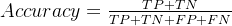
- Accuracy(准确率)是最常用的指标,所有预测正确的占全部的比例
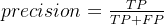
- Precision(精度,查准率)看的是在预测为真的情形下有多少是预测正确的,即「精准度」是多少
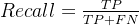
- Recall(召回率,查全率)是看在实际为真的情形中,预测「能召回多少」实际为真的答案
多分类示例
1.混淆矩阵
不想太麻烦,就随机生成了两组4 4的数据作为真实值b和预测值a,生成混淆矩阵。
#生成数据
import numpy as np
a = np.random.randint(0, 6, size=(4,4))#预测值
b = np.random.randint(0, 6, size=(4,4))#真实值
n = 6
print(a)
print(b)

#生成混淆矩阵
def fast_hist(a, b, n):
    k = (b >= 0) & (b < n)
    # 横坐标是预测的类别,纵坐标是真实的类别
    #n_class * label_true[mask].astype(int) + label_pred[mask]计算得到的是二维数组元素变成一维度数组元素的时候的地址取值(每个元素大小为1),返回的是一个numpy的list,然后
    #np.bincount就可以计算各中取值的个数
    hist = np.bincount(a[k].astype(int) + n*b[k].astype(int), minlength=n**2).reshape(n,n)
    return hist
print(fast_hist(a, b, n))
#随机生成的数据
[[4 2 2 0]
[5 1 1 3]
[4 0 2 1]
[1 1 4 1]]
[[3 4 5 0]
[2 4 5 1]
[4 0 1 0]
[1 4 2 4]]#混淆矩阵: 横坐标是预测的类别,纵坐标是真实的类别
[[2 1 0 0 0 0]
[0 1 1 1 0 0]
[0 0 0 0 1 1]
[0 0 0 0 1 0]
[0 3 1 0 1 0]
[0 1 1 0 0 0]]
2.iou(交并比)
def per_class_iou(hist):
    """
    hist传入混淆矩阵(n, n)
    """
    # 因为下面有除法,防止分母为0的情况报错
    np.seterr(divide="ignore", invalid="ignore")
    # 交集:np.diag取hist的对角线元素
    # 并集:hist.sum(1)和hist.sum(0)分别按两个维度相加,而对角线元素加了两次,因此减一次
    iou = np.diag(hist) / (hist.sum(1) + hist.sum(0) - np.diag(hist))
    # 把报错设回来
    np.seterr(divide="warn", invalid="warn")
    # 如果分母为0,结果是nan,会影响后续处理,因此把nan都置为0
    iou[np.isnan(iou)] = 0.
    return iou
print(per_class_iou(hist))
#iou
[0.66666667 0.125 0. 0. 0.14285714 0. ]
miou
对iou求平均就是miou
miou = np.nanmean(iou)3.召回率
对角线上的数值(预测正确的真)比上hist每一行的和(每一类实际为真的数量)
#每一类的准确率
def per_class_acc(hist):
    """
    :param hist: 混淆矩阵
    :return: 每类的acc和平均的acc
    """
    np.seterr(divide="ignore", invalid="ignore")
    acc_cls = np.diag(hist) / hist.sum(1)   #改变hist.sum()的维度就是精度
    np.seterr(divide="warn", invalid="warn")
    acc_cls[np.isnan(acc_cls)] = 0.
    return acc_cls
print(per_class_acc(hist))
#每类的召回率
[0.66666667 0.33333333 0. 0. 0.2 0. ]
再求平均就是召回率了
4.acc(准确率)
预测正确的比上所有
acc = np.diag(hist).sum() / hist.sum()0.25
5.混淆矩阵可视化
# 绘制hist矩阵的可视化图并保存
def drawHist(hist, path):

    hist_ = hist
    hist_tmp = np.zeros((class_num, class_num))

    for i in range(len(hist_)):
        hist_tmp[i] = hist_[i]

    print(hist_tmp)
    hist = hist_tmp
    plt.matshow(hist)
    plt.xlabel("Predicted label")
    plt.ylabel("True label")
    plt.axis("off")
    # plt.colorbar()
    plt.show()
    if (path != None):
        plt.savefig(path)
        print("%s保存成功✿✿ヽ(°▽°)ノ✿" % path)
完整代码
import torch
import numpy as np
import matplotlib.pyplot as plt


# 计算各种评价指标
def fast_hist(a, b, n):
    """
    生成混淆矩阵
    a 是形状为(HxW,)的预测值
    b 是形状为(HxW,)的真实值
    n 是类别数
    """
    # 确保a和b在0~n-1的范围内,k是(HxW,)的True和False数列
    k = (a >= 0) & (a < n)
    # 横坐标是预测的类别,纵坐标是真实的类别
    hist = np.bincount(a[k].astype(int) + n * b[k].astype(int), minlength=n ** 2).reshape(n, n)
    return hist


def per_class_iou(hist):
    # 因为下面有除法,防止分母为0的情况报错
    np.seterr(divide="ignore", invalid="ignore")
    # 交集:np.diag取hist的对角线元素
    # 并集:hist.sum(1)和hist.sum(0)分别按两个维度相加,而对角线元素加了两次,因此减一次
    iou = np.diag(hist) / (hist.sum(1) + hist.sum(0) - np.diag(hist))
    # 把报错设回来
    np.seterr(divide="warn", invalid="warn")
    # 如果分母为0,结果是nan,会影响后续处理,因此把nan都置为0
    iou[np.isnan(iou)] = 0.
    return iou


def per_class_acc(hist):
    """
    :param hist: 混淆矩阵
    :return: 每类的acc和平均的acc
    """
    np.seterr(divide="ignore", invalid="ignore")
    acc_cls = np.diag(hist) / hist.sum(1)
    np.seterr(divide="warn", invalid="warn")
    acc_cls[np.isnan(acc_cls)] = 0.
    return acc_cls


# 使用这个函数计算模型的各种性能指标
# 输入网络的输出值和标签值,得到计算结果
def get_MIoU(pred, label, hist):
    """
    :param pred: 预测向量
    :param label: 真实标签值
    :return: 准确率,每类的准确率,每类的iou, miou
    """
    hist = hist
    # 准确率
    acc = np.diag(hist).sum() / hist.sum()
    # 每一类的召回率
    acc_cls = per_class_acc(hist)
    # 每类的iou
    iou = per_class_iou(hist)
    # miou
    miou = np.nanmean(iou[1:])
    return acc, acc_cls, iou, miou, hist


# 绘制hist矩阵的可视化图并保存
def drawHist(hist, path):
    # print(hist)
    hist_ = hist
    hist_tmp = np.zeros((n, n))

    for i in range(len(hist_)):
        hist_tmp[i] = hist_[i]

    print(hist_tmp)
    hist = hist_tmp
    plt.matshow(hist)
    plt.xlabel("Predicted label")
    plt.ylabel("True label")
    plt.axis("off")
    # plt.colorbar()
    plt.show()
    if (path != None):
        plt.savefig(path)
        print("%s保存成功✿✿ヽ(°▽°)ノ✿" % path)


if __name__ == "__main__":
    # 随机生成数据
    a = np.random.randint(0, 6, size=(4, 4))
    b = np.random.randint(0, 6, size=(4, 4))
    n = 6
    hist = fast_hist(a, b, n)
    print(a)
    print(b)
    print(get_MIoU(a, b, hist))

    drawHist(hist, "C:/Users/Administrator/Desktop")
#所有结果
[[5 1 5 0]
[4 0 5 1]
[2 4 2 1]
[1 3 2 5]]
[[0 3 3 3]
[1 2 0 1]
[0 3 1 1]
[5 5 3 5]]
(0.1875, array([0. , 0.5 , 0. , 0. , 0. ,
0.33333333]), array([0. , 0.33333333, 0. , 0. , 0. ,
0.16666667]), 0.1, array([[0, 0, 1, 0, 0, 2],
[0, 2, 1, 0, 1, 0],
[1, 0, 0, 0, 0, 0],
[1, 1, 1, 0, 1, 1],
[0, 0, 0, 0, 0, 0],
[0, 1, 0, 1, 0, 1]], dtype=int64))
[[0. 0. 1. 0. 0. 2.]
[0. 2. 1. 0. 1. 0.]
[1. 0. 0. 0. 0. 0.]
[1. 1. 1. 0. 1. 1.]
[0. 0. 0. 0. 0. 0.]
[0. 1. 0. 1. 0. 1.]]