em算法和gmm算法_ml gmm em算法

GMM is a really popular clustering method you should know as a data scientist. K-means clustering is also a part of GMM. GMM can overcome the limitation of k-means clustering. In this post, I will explain how GMM works and how it will be trained.

GMM是一种非常流行的群集方法，您应该作为数据科学家知道。 K均值聚类也是GMM的一部分。 GMM可以克服k均值聚类的局限性。 在这篇文章中，我将解释GMM的工作原理以及培训方法。

混合模型 (Mixture Model)

What is the mixture model? We can think of just the combination of the models. If you combine the Gaussian Distribution with weights, then it will be the Gaussian Mixture Model. The pi in the equations is the weight, mixing coefficient, of the model, the sum of every weight should be 1 because the probability cannot over 1. It also should be between 0 and 1.

什么是混合模型？ 我们可以想到的只是模型的组合。 如果将高斯分布与权重结合起来，那么它将是高斯混合模型。 方程中的pi是模型的权重，混合系数，每个权重的总和应为1，因为概率不能超过1。它也应在0到1之间。

Each of the normal distribution in the mixture has its own mean parameter and covariance parameter.

混合物中的每个正态分布都有自己的平均参数和协方差参数。

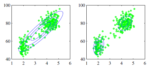
Why do we need the mixture model? It is clear if you watch the above picture. The Gaussian should be dense around the mean but it is not. If we want to fit this properly, we need two Gaussian models, clustering.

为什么需要混合模型？ 很明显，如果您观看上面的图片。 高斯应该在均值周围密集，但事实并非如此。 如果我们想适当地拟合它，我们需要两个高斯模型，即聚类。

We can also overlap the Gaussian to fit the data. The numbers next to the gaussian in the left graph are weight. The right picture shows the fitted density with a 3D image.

我们还可以重叠高斯来拟合数据。 左图中高斯旁边的数字是权重。 右图显示了3D图像的拟合密度。

生成模型 (Generative model)

We can use GMM as a Generative Model. If you select the components and you know the parameter of the corresponding gaussian, then you can sample from the Gaussian. Actually, now we can change our minds. It is somehow intuitive and tricky.

我们可以将GMM用作生成模型。 如果选择组件并且知道相应高斯的参数，则可以从高斯采样。 实际上，现在我们可以改变主意了。 这有点直观和棘手。

Can we think the pi, weight, as a probability? Yes, we can. What does it mean? It means how likely we choose a specific model, it can be interpreted as how likely we choose a specific parameter set of the Gaussian distribution. Then,

我们可以将圆周率，权重视为概率吗？ 我们可以。 这是什么意思？ 这意味着我们选择特定模型的可能性有多高，可以解释为我们选择高斯分布的特定参数集的可能性有多大。 然后，

This will be a likelihood. Zn is a categorical variable.

这将是可能的。 Zn是分类变量。

We can calculate the probability of the specific data like above. This is the equivalent generative formulation with an explicit latent variable Zn. We can illustrate this.

我们可以像上面那样计算特定数据的概率。 这是具有明显潜变量Zn的等效生成公式。 我们可以举例说明。

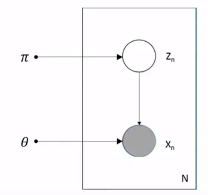
The shaded circle is the observed data. If we know pi, we can generate Zn. If we know Zn, we can generate new data. In our case, it is Gaussian distribution but it can be any distribution you want.

阴影圆圈是观察到的数据。 如果我们知道pi，就可以生成Zn。 如果我们知道Zn，就可以生成新数据。 在我们的例子中，它是高斯分布，但也可以是您想要的任何分布。

Let’s look at this with bayesian eyes. If you don’t familiar with it, you can check here.

让我们用贝叶斯的眼睛看一下。 如果您不熟悉它，可以在这里查看。

I already define the likelihood above and we define other things here. We want to calculate the posterior, it means what is the probability of the parameter given data from component k, specific gaussian distribution. The posterior is also called responsibility. We can understand this as the specific data group how likely to be assigned in the specific class. However, Gaussians contribute to every data point with weight, we need to compare this with every other Gaussians. We can calculate this with Bayes’s rule.

我已经在上面定义了可能性，我们在这里定义了其他内容。 我们要计算后验，这意味着给定来自分量k的数据，特定的高斯分布的参数的概率是多少。 后方也称为责任。 我们可以理解为特定数据组在特定类别中的分配可能性。 但是，高斯人对每个数据点的贡献都很大，我们需要将其与其他所有高斯人进行比较。 我们可以用贝叶斯定律来计算。

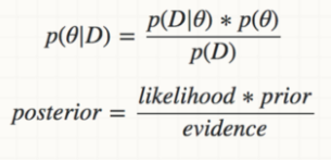
Posterior is calculated by multiplying likelihood and prior and evidence is constant.

后验是通过将可能性与先验相乘得出的，并且证据是恒定的。

We assign the data point into the class where it has the biggest responsibility and color it. It will look like this. However, you should check the last picture has a blurred area where we cannot decide which cluster is the right cluster.

我们将数据点分配给责任最大的类并为其着色。 它看起来像这样。 但是，您应该检查最后一张图片的模糊区域，在该区域我们无法确定哪个群集是正确的群集。

参数估计 (Parameter Estimation)

We need to find out the covariance matrix, mixing coefficient, and mean vector. First of all, we assume that we know the K. I will explain how to choose k later. It is difficult to calculate because of the covariance matrix, it is p by p size. We assume i.i.d and we can conclude the likelihood is:

我们需要找出协方差矩阵，混合系数和均值向量。 首先，我们假设我们知道K。稍后我将解释如何选择k。 由于协方差矩阵，很难计算，它是p x p大小。 我们假设iid，我们可以得出结论是：

The log-likelihood will be:

对数似然将是：

If you are familiar with other log-likelihoods, you can feel weird in this equation because it is hard to differentiate the function. This is a problematic part of the parameter estimation. If you just go for it, you can get this equation, we set the derivative to zero:

如果您熟悉其他对数似然，则由于很难区分该函数，因此您可能会觉得这个方程式很奇怪。 这是参数估计的有问题的部分。 如果您只是这样做，则可以得到以下等式，我们将导数设置为零：

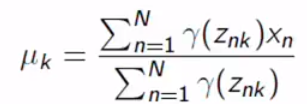
If you differentiate it by yourself, you can get the responsibility term. The equation above contains responsibility terms. We still can not calculate the mean because we don’t know the responsibility, it contains every parameter. We can do something for covariance.

如果您自己进行区分，则可以获得责任条款。 上面的等式包含责任条款。 我们仍然无法计算均值，因为我们不知道责任，它包含每个参数。 我们可以做一些协方差。

Same result for pi.

pi的结果相同。

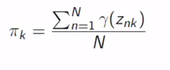
How do we solve this? We can do it by setting the initial parameter and calculate the log-likelihood and update the parameters with respect to responsibility, we can get it because we initialized the parameters. Repeat this until convergence. This is called the EM method.

我们该如何解决呢？ 我们可以通过设置初始参数并计算对数似然率并根据责任更新参数来完成此操作，因为初始化了参数，所以可以得到它。 重复此步骤直到收敛。 这称为EM方法。

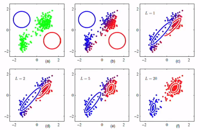
期望最大化 (Expectation Maximization)

This is one way to do maximum likelihood estimation when you have missing data. EM is an iterative algorithm.

这是丢失数据时进行最大似然估计的一种方法。 EM是一种迭代算法。

0. Initialize the parameters and evaluate the log-likelihood.

0.初始化参数并评估对数可能性。

1. Compute the Posterior distribution of Z gives current estimator of parameters:
   计算Z的后验分布可得出参数的当前估计值：

2. Compute Complete likelihood under this distribution of Z (Expectation):

2.计算此Z分布(期望)下的完全似然：

3. We maximize this Q functions(Maximization):

3.我们最大化这个Q函数(Maximization)：

What the algorithm does is simple. We don’t know the Z. We built the distribution, in GMM, the responsibility based on previous guesses, about Z, hidden variables, based on the previous guess. We calculate the expected value of complete log-likelihood under the distribution of the missing data using the previous guess, Expectation Step, and we maximize it with respect to the parameters for the next parameter, Maximization Step.

该算法的作用很简单。 我们不知道Z。我们在GMM中建立了基于先前猜测的责任分布，基于先前的猜测关于Z和隐藏变量。 我们使用先前的猜测(期望步长)在缺失数据的分布下计算完全对数似然的期望值，并针对下一个参数(最大化步长)将其最大化。

GMM的期望最大化 (Expectation-Maximization for GMM)

We assume that hidden variables and latent variables are equal. What we are finding now is covariance, mixing coefficient, and mean.

我们假设隐藏变量和潜在变量相等。 我们现在发现的是协方差，混合系数和均值。

Again, you have to remember the important point in the E step, we calculate the expected value of complete log-likelihood under the Z distribution using the previous guess.

同样，您必须记住E步骤中的要点，我们使用先前的猜测来计算Z分布下完全对数似然的期望值。

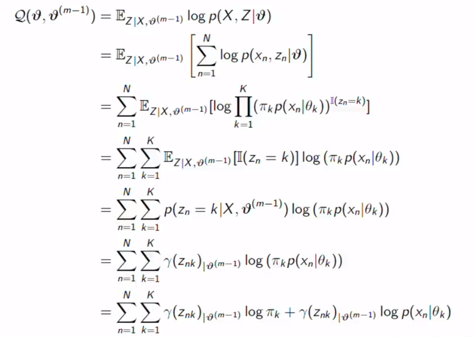
Now, we still got the responsibility. However, it is not about the true parameter. It is the responsibility based on guessed parameters. The equation is also easy to differentiate for M step.

现在，我们仍然有责任。 但是，这与true参数无关。 这是基于猜测参数的责任。 该方程对于M步也很容易微分。

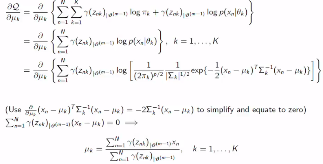
Responsibility becomes constant.

责任变得恒定。

Same for other parameters.

其他参数相同。

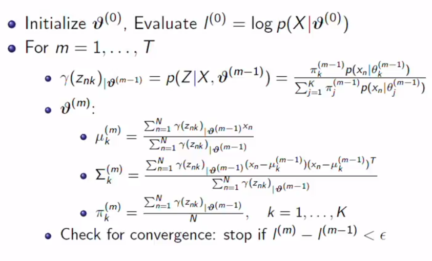
This is the whole picture of EM for GMM.

这是EM for GMM的整体情况。

理论保证 (Theoretical Guarantee)

EM monotonically increases observed data likelihood until the local maximum or saddle point. Let’s look at why it is the case. The context you should know is Jansen’s inequality. If we have convex function f, then:

EM单调增加观察到的数据的可能性，直到局部最大值或鞍点。 让我们看看为什么会这样。 您应该知道的上下文是Jansen不等式。 如果我们有凸函数f，则：

The function of the linear combination of x will less than a linear combination of functions of x. What we need is when f is a log, concave function. It will be the opposite.

x的线性组合的函数将小于x的线性函数的组合。 我们需要的是f是对数凹函数。 相反。

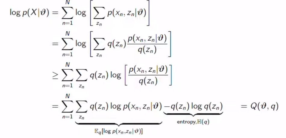
We calculate the log-likelihood but now we set q as an arbitrary distribution over the latent variables. We got lower bound with Jansen’s Inequality. Finally, we get the Q function, we got the expected value of log-likelihood minus entropy. We need to choose q to maximize the Q function. To sum up, we maximize the lower bound to touch the original likelihood.

我们计算对数似然，但现在我们将q设置为潜在变量的任意分布。 Jansen不等式的下界。 最后，我们得到Q函数，得到对数似然减去熵的期望值。 我们需要选择q以最大化Q函数。 综上所述，我们将下限最大化以触及原始可能性。

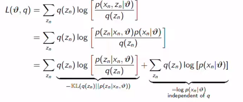
I changed the lower bound formula into -KL divergence + Log-likelihood. Our goal is to make KL divergence zero because we want to consider log-likelihood. It turns out EM did the same process, making KL divergence zero.

我将下限公式更改为-KL散度+对数似然。 我们的目标是使KL散度为零，因为我们要考虑对数似然。 事实证明，EM执行了相同的过程，从而使KL散度为零。

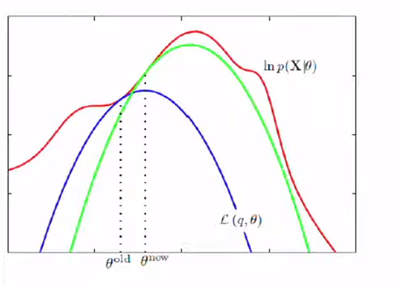
This picture tells the process.

此图说明了过程。

BIC和AIC (BIC & AIC)

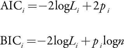
These are the popular information criterion, you can use both in general. We will use this to choose K in GMM. AIC consists of log-likelihood, which we maximized for a good model and the number of parameters, k in our case. We penalized the loglikelihood with the number of parameters because many parameters can lead to the perfect model but it is definitely overfitting. BIC is almost the same but it has weight for the number of parameters, a log of the number of observed data. More data, more penalty. This is not good to build a complex model even if you have enough data.

这些是流行的信息准则，一般可以同时使用。 我们将使用它在GMM中选择K。 AIC包含对数似然性，对于一个好的模型和参数数量(在本例中为k)，我们将其最大化。 我们用参数数量来惩罚对数似然性，因为许多参数可以得出理想的模型，但绝对过拟合。 BIC几乎相同，但是它具有权重参数数量，即观察到的数据数量的对数。 更多数据，更多惩罚。 即使您有足够的数据，也很难建立一个复杂的模型。

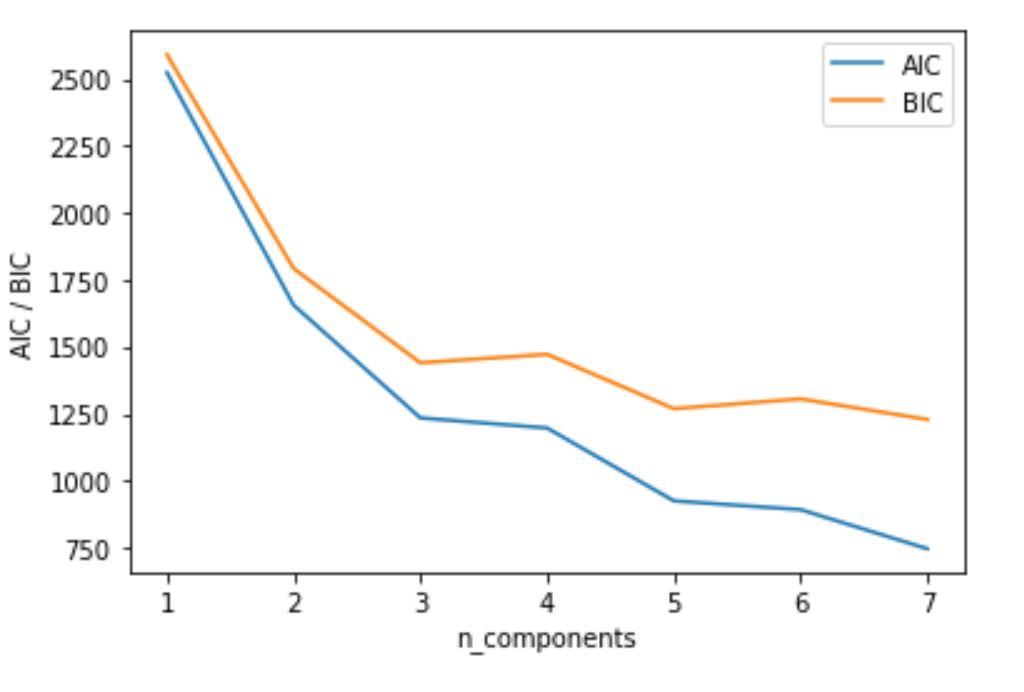
In this graph, I would like to say 3, 5 are a nice choice for k because the model is not that complex and nice AIC and BIC score.

在此图中，我想说3、5是k的不错选择，因为该模型不是那么复杂且不错的AIC和BIC得分。

协方差类型 (Covariance Types)

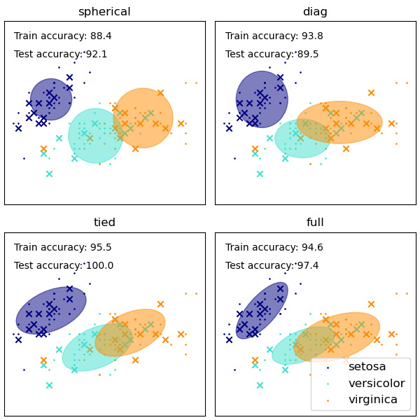
We can have different types of Gaussian distribution depending on the covariance matrices. If the covariance is always the same in every direction, then it will be spherical. It is a diagonal matrix but the same variances. You should know they don’t share the same covariance. The diagonal means the covariance matrix is diagonal but it is not the same. Tied means they share the covariance together.

根据协方差矩阵，我们可以具有不同类型的高斯分布。 如果协方差在每个方向上始终相同，那么它将是球形的。 它是对角矩阵，但方差相同。 您应该知道它们不具有相同的协方差。 对角线表示协方差矩阵是对角线，但不相同。 并列表示他们共同共享协方差。

This post is published on 9/24/2020.

此帖发布于9/24/2020。