[论文精读]Dynamic Coarse-to-Fine Learning for Oriented Tiny Object Detection
论文网址:[2304.08876] 用于定向微小目标检测的动态粗到细学习 (arxiv.org)
论文代码:https://github.com/ChaselTsui/mmrotate-dcfl
英文是纯手打的!论文原文的summarizing and paraphrasing。可能会出现难以避免的拼写错误和语法错误,若有发现欢迎评论指正!文章偏向于笔记,谨慎食用
1. 省流版
1.1. 心得
(1)为什么学脑科学的我要看这个啊?愿世界上没有黑工
(2)最开始写小标题的时候就发现了,分得好细啊,好感度++
(3)作为一个外行人,这文章感觉提出了好多东西
1.2. 论文总结图
2. 论文逐段精读
2.1. Abstract
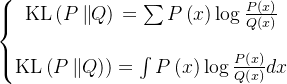
①Extreme geometric shapes (tiny) and finite features (few pixels) of tiny rotating objects will cause serious mismatch (inaccurate positional prior?) and imbalance (inaccurate positive sample features?) issues
②They proposed dynamic prior and coarse-to-fine assigner, called DCFL
posterior adj.在后部的;在后面的 n.臀部;屁股
2.2. Introduction
①Oriented bounding box greatly eliminates redundant background area, especially in aerial images
②Comparison figure:
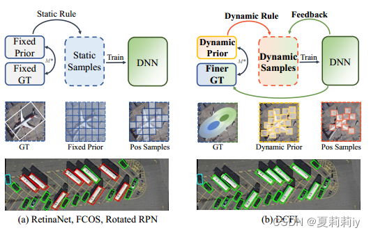
where M* denotes matching function;
green, blue and red boxes are true positive, false positive, and false negative predictions respectively,
the left figure set is static and the right is dynamic
③Figure of mismatch and imbalance issues:
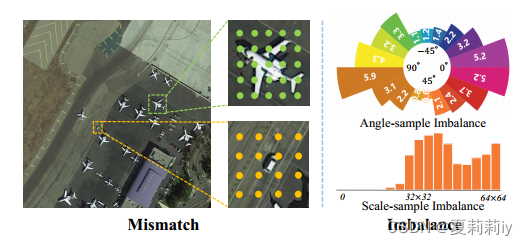
each point in the left figure denotes a prior location(先验打那么多个点啊...而且为啥打得那么整齐,这是什么one-stage吗)
饼状图是说当每个框都是某个角度的时候吗?当每个框都不旋转的时候阳性样本平均数量是5.2?还是说饼状图的意思是自由旋转,某个特定角度的框的阳性样本是多少多少?这个饼状图并没有横向比较诶,只有这张图自己内部比较。
柱状图是锚框大小不同下平均阳性
④They introduce dynamic Prior Capturing Block (PCB) as their prior method. Based on this, they further utilize Cross-FPN-layer Coarse Positive Sample (CPS) to assign labels. After that, they reorder these candidates by prediction (posterior), and present gt by finer Dynamic Gaussian Mixture Model (DGMM)
eradicate vt.根除;消灭;杜绝 n.根除者;褪色灵
2.3. Related Work
2.3.1. Oriented Object Detection
(1)Prior for Oriented Objects
(2)Label Assignment
2.3.2. Tiny Object Detection
(1)Multi-scale Learning
(2)Label Assignment
(3)Context Information
(4)Feature Enhancement
2.4. Method
(1)Overview
①For a set of dense prior  , where
  denotes width,
  denotes height and
  denotes the number of shape information(什么东西啊,是那些点吗), mapping it to
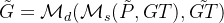
  by Deep Neural Network (DNN):
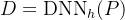
where  represents the detection head(探测头...外行不太懂,感觉也就是一个函数嘛?);
one part 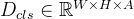 in
in  denotes the classification scores, where
  means the class number(更被认为是阳性的样本那层的
 里的数据会更大吗);
one part  in
in  denotes the classification scores, where
  means the box parameter number(查宝说是w, h, x, y, a之类的是box parameter)
②In static methods, the pos labels assigned for  is
is 
③In dynamic methods, the pos labels set  integrate posterior information:
④The loss function:

where  and
and  represent the number of positive and negative samples,
  is the neg labels set
⑤Modelling  ,
,  and
and  :
:

2.4.1. Dynamic Prior
①Flexibility may alleviate mismatch problem
②Each prior represents a feature point
③The structure of Prior Capturing Block (PCB):
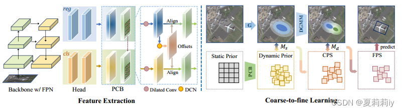
the surrounding information is considered by dilated convolution. Then caputure dynamic prior by Deformable Convolution Network (DCN). Moreover, using the offset learned from the regression branch to guide feature extraction in the classification branch and improve alignment between the two tasks.
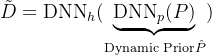
④To achieve dynamic prior capturing, initializing each prior loaction  by each feature point’s spatial location
  . In each iteration, capture the offset set of each prior position
  to update
  :
:
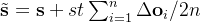
where  denotes the stride of feature map,
  denotes the number of offsets;
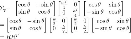
2D Gaussian distribution  is regarded as the prior distribution;
动态的 作为高斯的平均向量
 (啥玩意儿??);
⑤Presetting a square  on each feature point
⑥The co-variance matrix:
dilate v.扩张;(使)膨胀;扩大 deformable adj.可变形的;应变的;易变形的
2.4.2. Coarse Prior Matching
①For prior, limiting  to a single FPN may cause sub-optimal layer selection and releasing
  to all layers may cause slow convergence
②Therefore, they propose Cross-FPN-layer Coarse Positive Sample (CPS) candidates, expanding candidate layers to  's nearby spatial location and adjacent FPN layers
③Generalized Jensen-Shannon Divergence (GJSD) constructs CPS between  and
and  :
:

which yields a closed-form solution;
where  ;
;
and due to the homogeneity of  and
and  ,
, 
④Choosing top  prior with highest GJSD for each
  (选差异最大的那些)
2.4.3. Finer Dynamic Posterior Matching
①Two main steps are contained in this section, a posterior re-ranking strategy and a Dynamic Gaussian Mixture Model (DGMM) constraint
②The Possibility of becoming True predictions (PT) of the  sample
  is:
is:

choosing top  samples with the highest scores as Medium Positive Sample (MPS) candidates
③They apply DGMM, which contains geometry center and semantic center in one object, to filter far samples
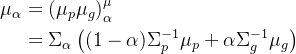
④For specific instance  , the mean vector
  of the first Gaussian is the geometry center
  , the deduced
  in MPS denotes semantic center
⑤Parameterizing a instance:

where  denotes weight of each Gaussian distribution and their summation is 1;
 equals to
  's
's  (什么啊这是,但是m可以等于1或者2诶,那你g的协方差不就又是语义中心又是几何中心了吗)
⑥For any  , setting negative masks
2.5. Experiments
2.5.1. Datasets
①Datasets: DOTAv1.0 /v1.5/v2.0, DIOR-R, VisDrone, and MS COCO
②Ablation dataset: DOTA-v2.0 with the most numbet of tiny objects
③Comparing dataset: DOTA-v1.0, DOTAv1.5, DOTA-v2.0, VisDrone2019, MS COCO and DIOR-R
2.5.2. Implementation Details
①Batch size: 4
②Framework based: MMDetection and MMRotate
③Backbone: ImageNet pre-trained models
④Learning rate: 0.005 with SGD
⑤Momentum: 0.9
⑥Weight decay: 0.0001
⑦Default backbone: ResNet-50 with FPN
⑧Loss: Focal loss for classifying and IoU loss for regression
⑨Data augmentation: random flipping
⑩On DOTA-v1.0 and DOTA-v2.0, using official setting to crop images to 1024×1024. The overlap is 200 and epoch is 12
⑪On other datasets, setting the input size to 1024 × 1024 (overlap 200), 800 × 800, 1333 × 800, and 1333×800 for DOTA-v1.5, DIOR-R, VisDrone, and COCO respectively. Epoch is set as 40, 40, 12, and 12 on the DOTA-v1.5, DIOR-R, COCO, and VisDrone
2.5.3. Main Results
(1)Results on DOTA series
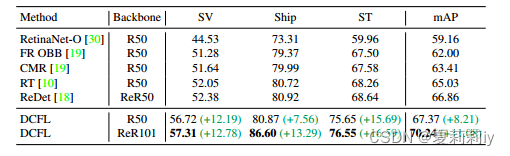
①Comparison table on DOTA-v2.0 OBB:
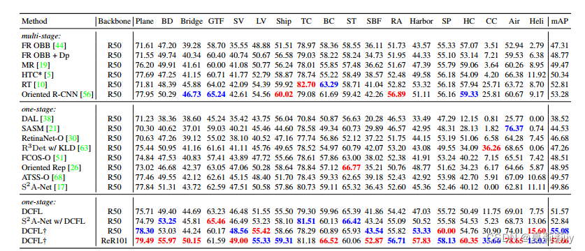
where the red ones are the best and the blue ones are the second best performance on each metric
②Comparison table on DOTA-v1.0 OBB:
③Comparison table on DOTA-v1.5 OBB:
(2)Results on DIOR-R
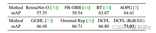
①Comparison table on DIOR-R:
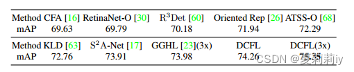
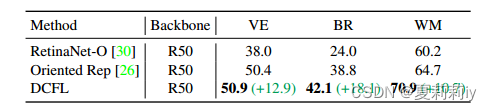
②Results of typical tiny objects vehicle, bridge, and wind-mill:
(3)Results on HBB Datasets
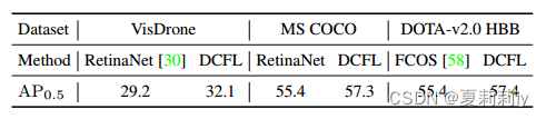
①Comparison table on VisDrone, MS COCO abd DOTA-v2.0 HBB:
2.5.4. Ablation Study
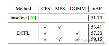
(1)Effects of Individual Strategy
①Employ prior on each feature point
②Individual effectiveness:
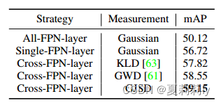
(2)Comparisons of Different CPS
①Ablation:
(3)Fixed Prior and Dynamic Prior
①Ablation:
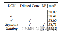
(4)Detailed Design in PCB
(5)Effects of Parameters
2.6. Analysis
(1)Reconciliation of imbalance problems
(2)Visualization
(3)Speed
2.7. Conclusion
3. 知识补充
4. Reference List
Xu, C. et al. (2023) 'Dynamic Coarse-to-Fine Learning for Oriented Tiny Object Detection', CVPR. doi: https://doi.org/10.48550/arXiv.2304.08876